Machine Learning Models Performance Evaluation
Model evaluation
In this section, you will learn about model evaluation. You will look at which metrics can be used for two very common ML algorithms: classification and regression.
Model evaluation datasets
Evaluation occurs after a model is trained. The data you use is partitioned into three parts: training set, validation set, and test set. The training set is used to train the model. The validation and test sets are the ones that you will use to evaluate the trained model performance.
Validation set
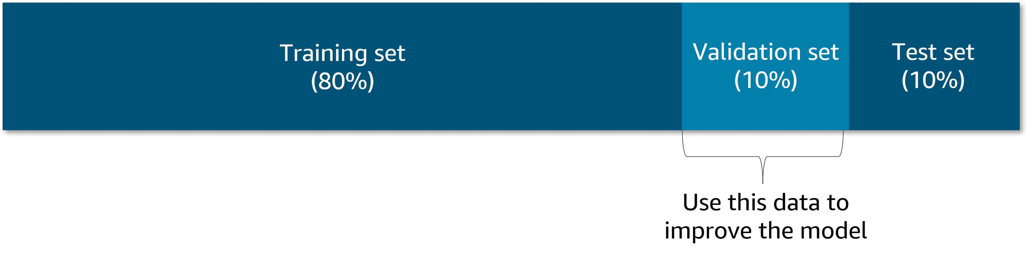
To begin evaluating how the model responds in a non-training environment, start by looking at the data that was set aside as the validation set. You want to make sure that the model generalizes to data it has not seen. The model still needs to be improved before determining that it’s ready for production.
Test set
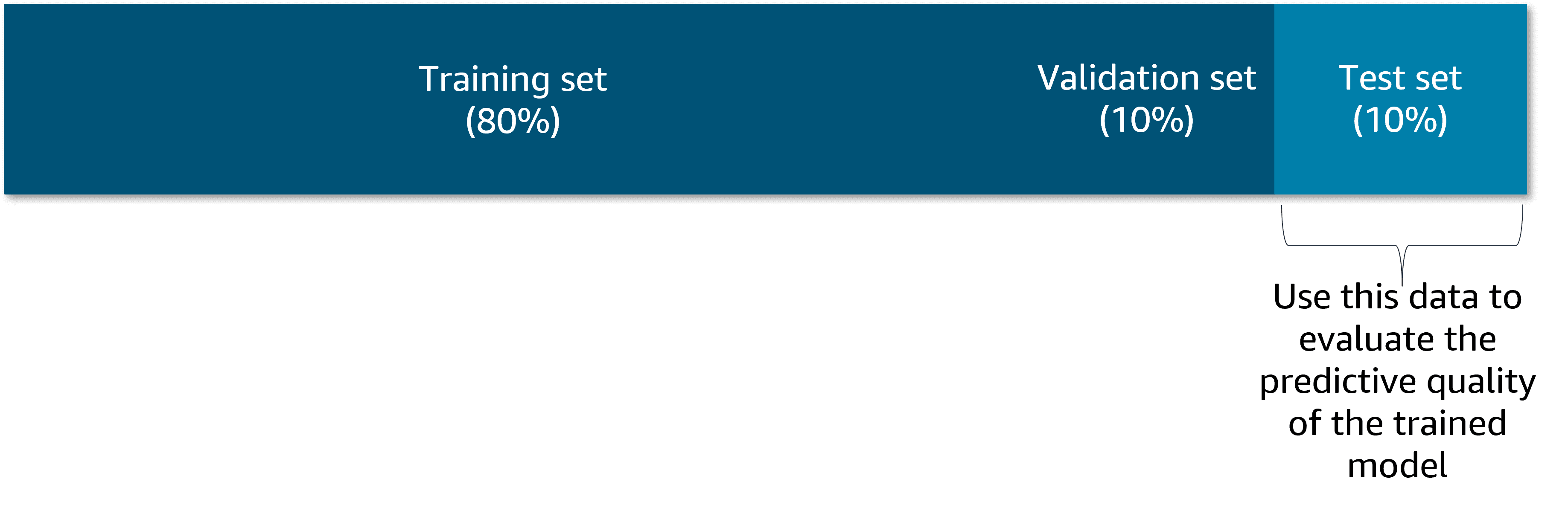
After you’ve improved the model using that validation data, you’re ready to test it one last time to ensure its predictive quality meets your standards.
Model fit
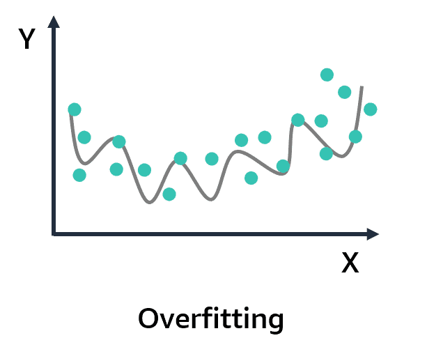
Model fit is important for understanding the root cause of poor model accuracy. This understanding will guide you to take corrective steps. You can determine whether a predictive model is underfitting or overfitting the training data by looking at the prediction error on the training data and the evaluation data.
Overfitting is when the model performs well on the training data but does not perform well on the evaluation data. This is because the model memorized the data it has seen and is unable to generalize to unseen examples.
Bias and variance
When evaluating models, both bias and variance contribute to errors the model makes on unseen data, which affects its generalization.
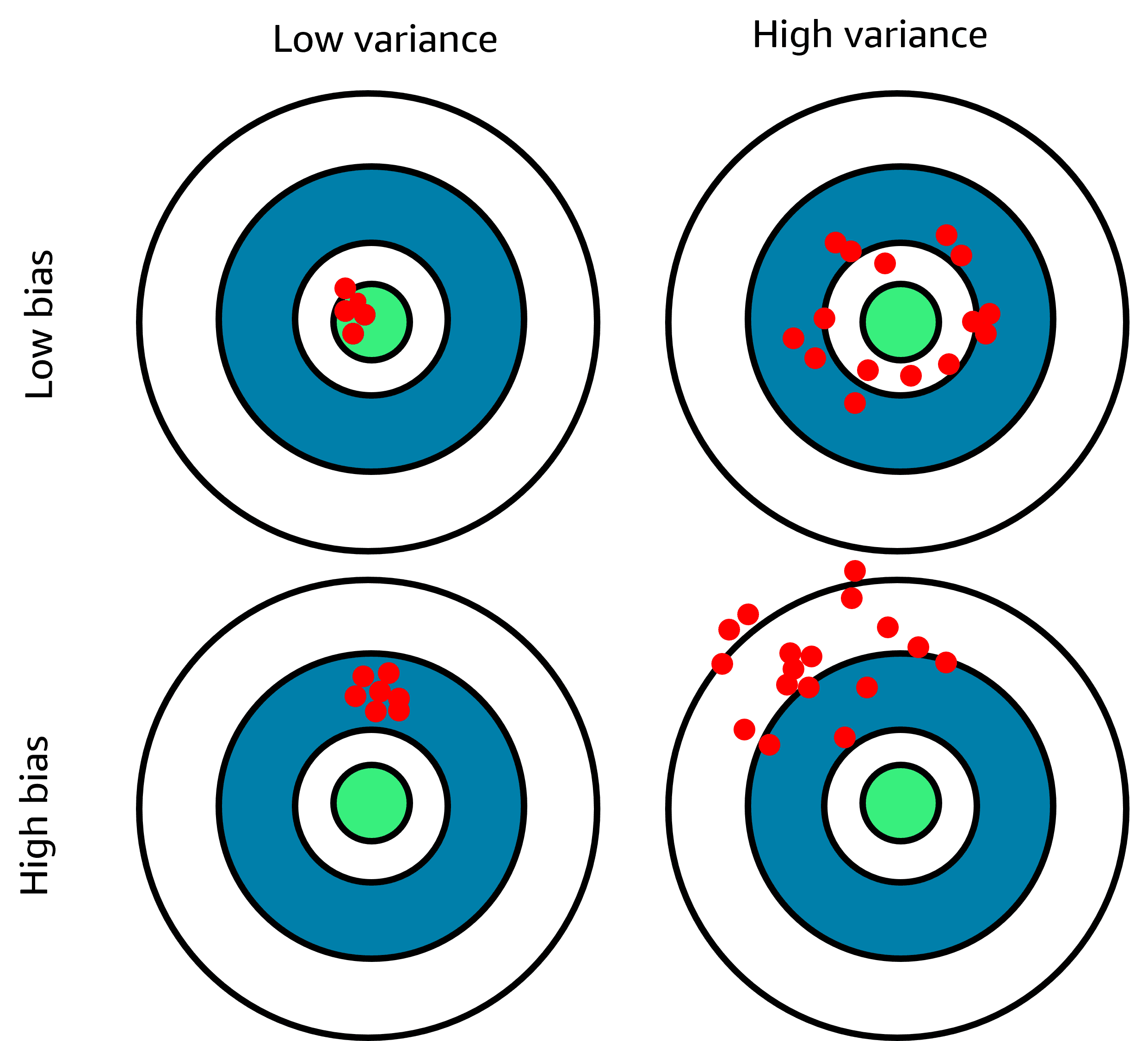
A bullseye is a nice analogy because, generally speaking, the center of the bullseye is where you aim your darts. The center of the bullseye in this situation is the label or target—it predicts the value of your model—and each dot is a result that your model produced during training.
Think about bias as the gap between your predicted value and the actual value, whereas variance describes how dispersed your predicted values are.
In ML, the ideal algorithm has low bias and can accurately model the true relationship. The ideal algorithm also has low variability, by producing consistent predictions across different datasets.
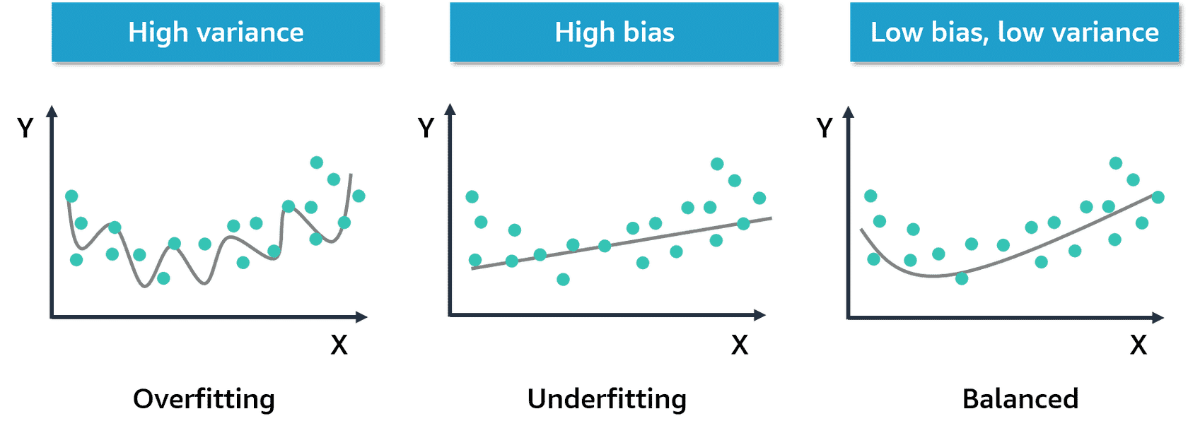
Balanced models have low bias and low variance
Classification and regression problems
How you evaluate a machine learning model depends on what kind of ML problem you're working with. In this section, you will look into the classification and regression metrics.
Classification metrics
- Accuracy
- Precision
- Recall
- F1
- AUC-ROC
Regression metrics
- Mean squared error
- R squared
Classification problem metrics
Classification example
The following is a binary classification problem where an image recognition model labels data as "cat" or "not cat."
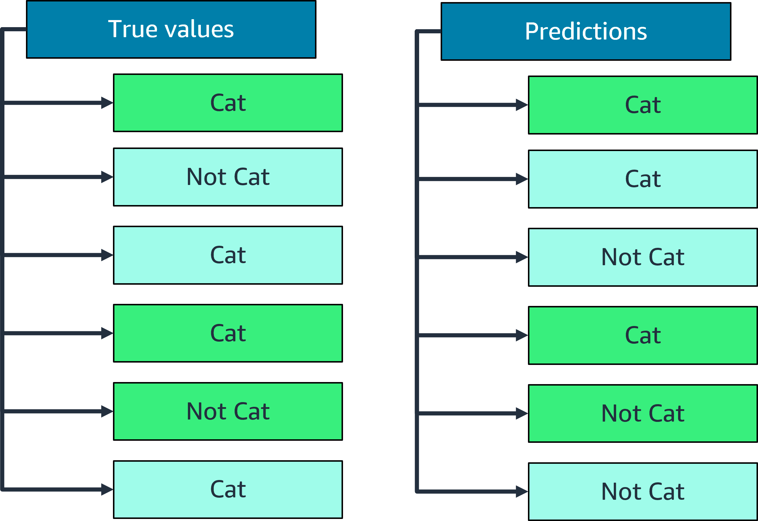
To evaluate a classification problem like the one shown, use the following steps:
Step 1: Send the held-out observations where you know the target values to the model.
Step 2: Compare the predictions returned by the model against the known target value.
Final Step: Compute a summary metric that shows how well the predicted and true values match.
Confusion matrix
A confusion matrix can help classify why and how a model gets something wrong. It is the building block for running these types of model evaluations for classification problems. Review the following graphic, which is a confusion matrix for the image recognition example. The matrix gives a high-level comparison of how the predicted classes matched up against the actual classes.
After the model has been applied to the testing data, each of the four boxes in the matrix will include an aggregate number of the unique occurrences of true positives, false positives, false negatives, and true negatives.
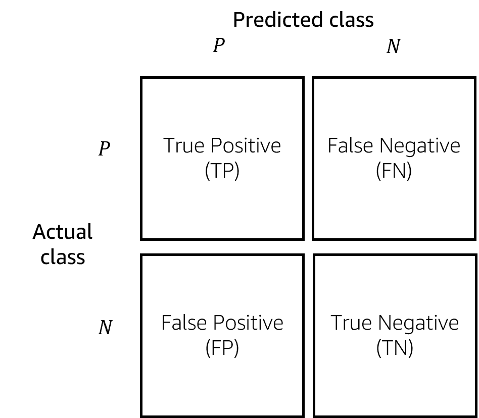
1: True positive (TP)
If the actual label or class is “cat,” which is identified as “P” for positive in the confusion matrix, and the predicted label or class is also “cat,” then you have a true positive result. This is a good outcome for your model.
Accuracy
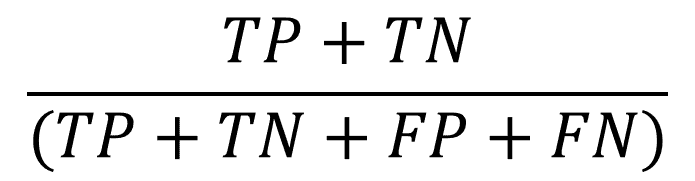
To calculate the model’s accuracy, also known as its score, add up the correct predictions and then divide that number by the total number of predictions.
| Although accuracy is a widely used metric for classification problems, it has limitations. This metric is less effective when there are a lot of true negative cases in your dataset. This is why two other metrics are often used in these situations: precision and recall. |
|---|
Precision
Precision removes the negative predictions from the picture. Precision is the proportion of positive predictions that are actually correct. You can calculate it by taking the true positive count and dividing it by the total number of positives.
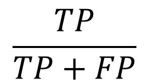
When the cost of false positives are high in your particular business situation, precision can be a good metric. Think about a classification model that identifies emails as spam or not. In this case, you do not want your model labeling a legitimate email as spam and preventing your users from seeing that email.
Recall
In addition to precision, there is also recall (or sensitivity). In recall, you are looking at the proportion of correct sets that are identified as positive. Recall is calculated by dividing the true positive count by the sum of the true positives and false negatives. By looking at that ratio, you get an idea of how good the algorithm is at detecting, for example, cats.
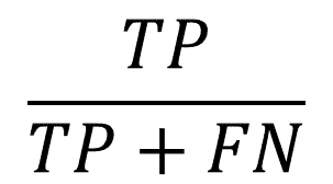
Think about a model that needs to predict whether a patient has a terminal illness or not. In this case, using precision as your evaluation metric does not account for the false negatives in your model. It is extremely important and vital to the success of the model that it not give false negative results. A false negative would be not identifying a patient as having a terminal illness when the patient actually does have a terminal illness. In this situation, recall is a better metric to use.
AUC-ROC
Area under the curve-receiver operator curve (AUC-ROC) is another evaluation metric. ROC is a probability curve, and AUC represents the degree or measure of separability.
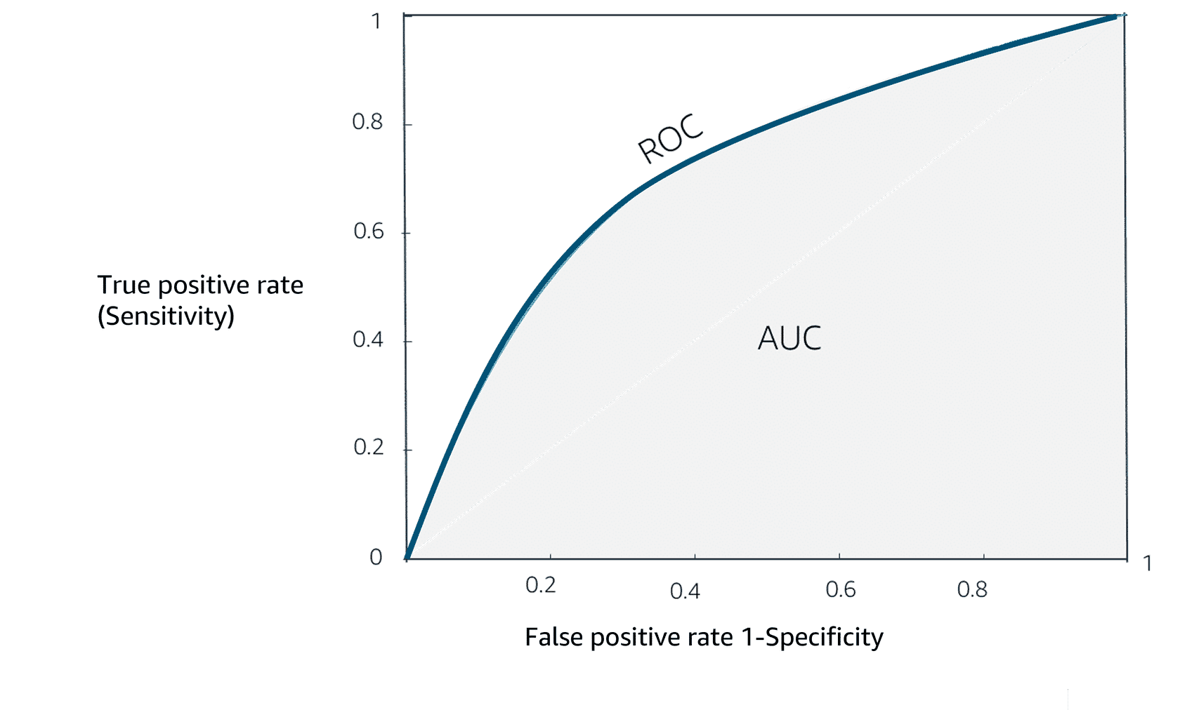
In general, AUC-ROC can show what the curve for true positive compared to false positive looks like at various thresholds. That means that when you calculate the AUC-ROC curve, you plot multiple confusion matrices at different thresholds and compare them to one another to find out the threshold you need for your business use case.
Example: Email spam classification
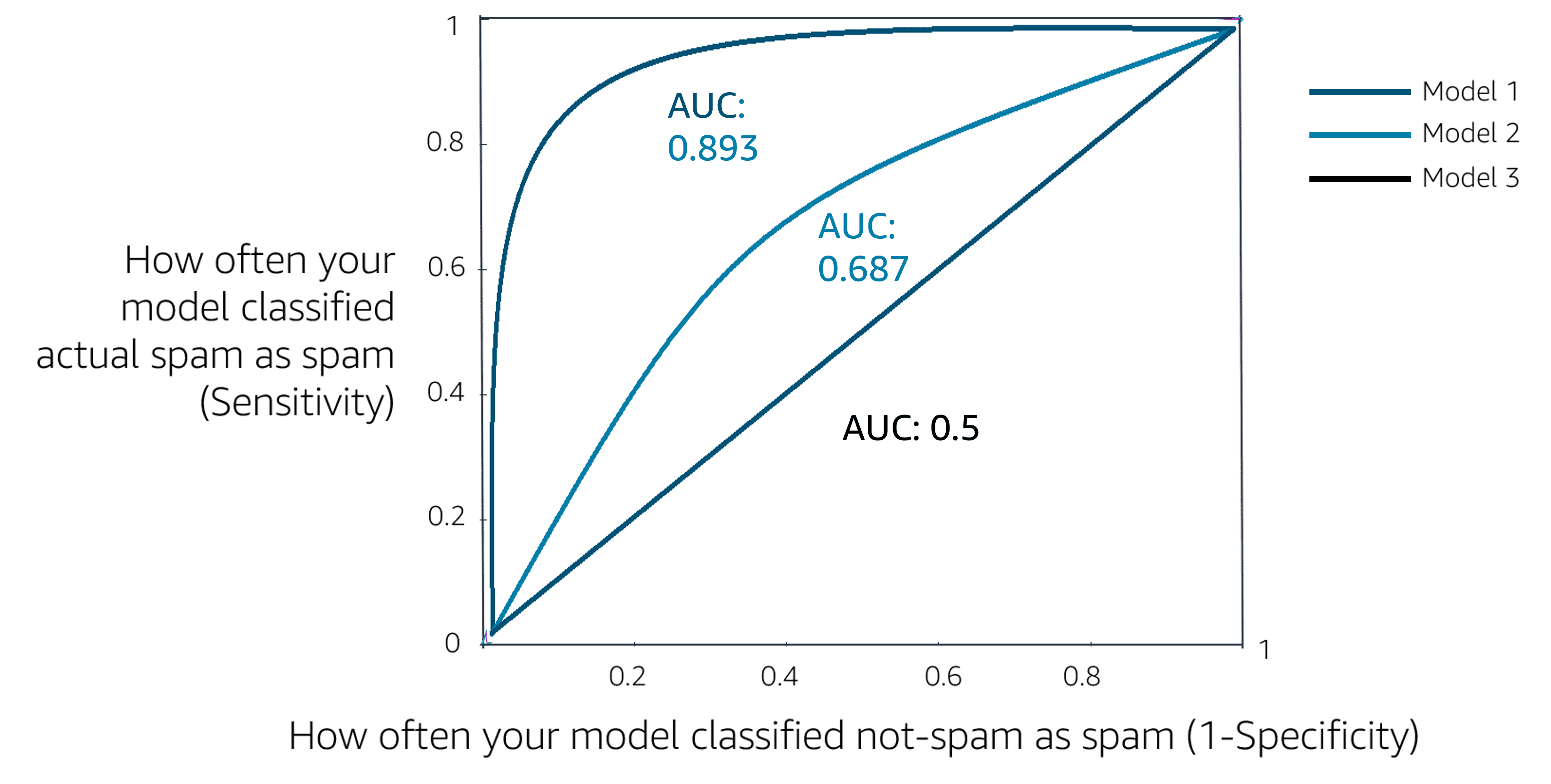
Take an example of email spam classification. The emails are rank ordered by the classifier’s risk score. In the following graph, high-scoring emails are on the left, and the vast majority of low-scoring emails are on the right.
1: X-axis
On the X-axis is the percentage of good emails that are going to be affected by your action—in this case, sidelining emails into spam folder.
Regression problem metrics
In case of a regression problem, there are other common metrics you can use to evaluate your model, including mean squared error and R squared. Mean squared error is very commonly used.
Mean squared error
The general purpose of mean squared error (MSE) is to evaluate regression model performance by measuring prediction accuracy. You determine the prediction from the model and compare the difference between the prediction and the actual outcome.
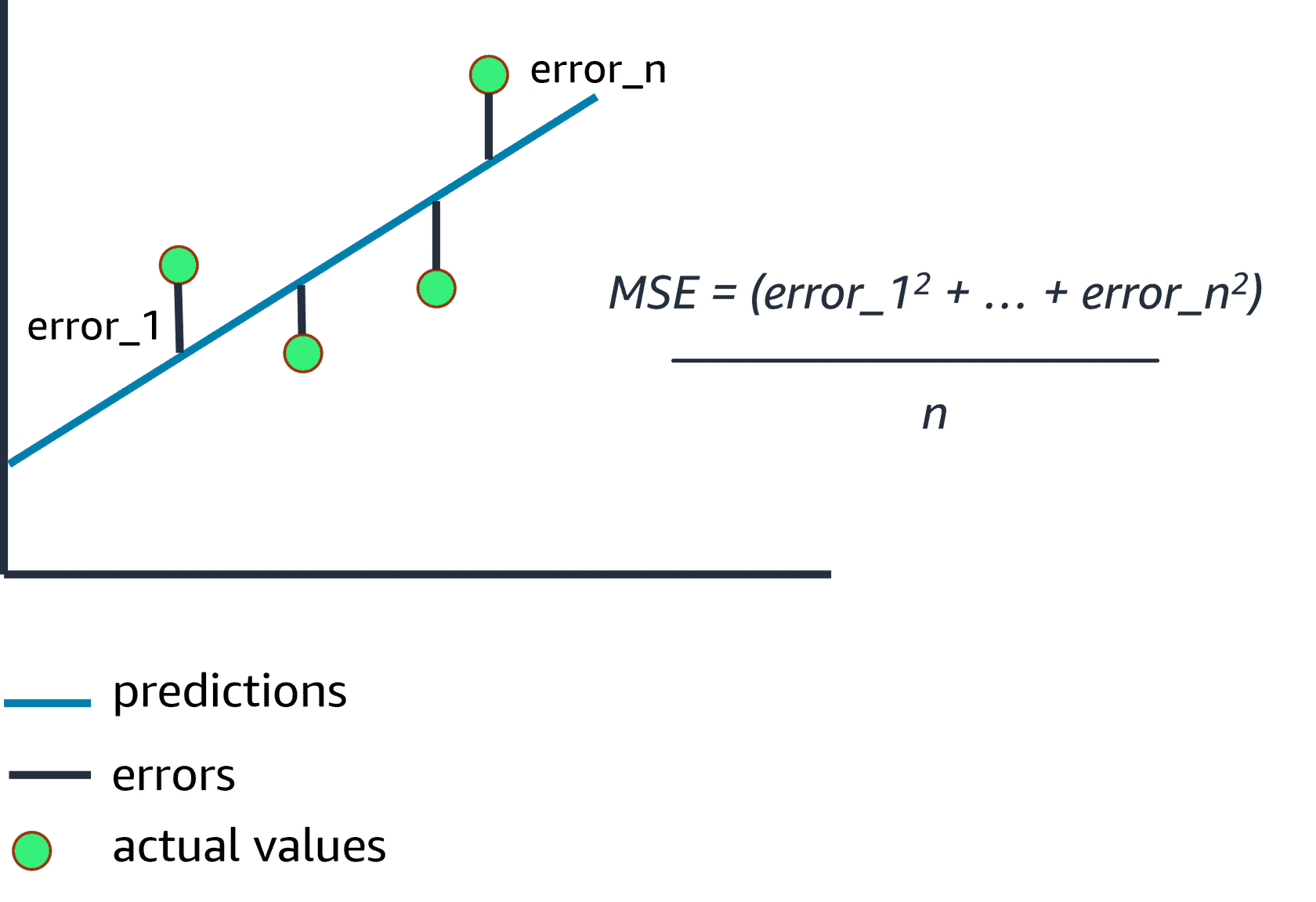
More specifically, you take the difference between the prediction and actual value, square that difference, sum up all the squared differences for all the observations, and then divide by the total number of observations to get the average.
The smaller the MSE, the better the model's predictive accuracy.
R squared
R squared is another commonly used metric with linear regression problems. R squared explains the fraction of variance accounted for by the model. It’s like a percentage, reporting a number from 0 to 1. When R squared is close to 1, it usually indicates that a lot of the variance in the data can be explained by the model itself.
MSE focuses on the average squared error of the model's predictions to provide a measure of model performance. R squared provides a measure of the model's goodness of fit to the data. Both are important but provide different perspectives.
Business metrics
In the previous section, you saw how to evaluate the performance of an ML model. But remember that when initiating a project, business set goals and KPIs are the metrics used to evaluate if the goals are met.
To validate and monitor model performance, establish numerical metrics that directly relate to the KPIs. These KPIs are established in the business goal identification phase. They can include goals such as increasing sales, cutting costs, or decreasing customer churn.
Evaluate whether the performance metrics accurately reflect the business’ tolerance for the error. For instance, false positives might lead to excessive maintenance costs in predictive maintenance use cases. Another example is deciding if acquiring a new customer is more expensive than retaining one. A business should focus on numerical metrics, such as precision and recall, to help differentiate the business requirements and be closer aligned to business value.
Consider developing custom metrics that tune the model directly for the business objectives. One way is to develop a cost function to evaluate the economic impact of the model. For the cost function, you can specify the cost, or value, of correct predictions and the cost of errors.
By using A/B testing or the canary deployments technique, developers can experiment with two or more variants of a model and help achieve the business goals.
In the next lesson, you will learn about Model deployment types